Non-Personalized Recommender systems with Pandas and Python

Hi all,

At the last PythonBrasil I gave a tutorial about Python and Data Analysis focused on recommender systems, the main topic I've been studying for the last years. There is a popular python package among the statisticians and data scientists called Pandas. I watched several talks and keynotes about it, but I didn't have a try on it. The tutorial gave me this chance and after the tutorial me and the audience fell quite excited about the potential and power that this library gives.

This post starts a series of articles that I will write about recommender systems and even the introduction for the new-old refreshed library that I am working on:  Crab,  a python library for building recommender systems. :)

This post starts with the first topic about the theme: Non-personalized Recommender Systems and giving several examples with the python package Pandas.  In future I will also post an alternative version of this post but referencing Crab, about how it works with him.

But first let's introduce what Pandas is.

Introduction to Pandas

Pandas is a data analysis library for Python that is great for data preparation, joining and ultimately generating well-formed, tabular data that's easy to use in a variety of visualization tools or (as we will see here) machine learning applications. For further introduction about pandas, check this website or this notebook.

Non-personalized Recommenders

Non-personalized recommenders can  recommend items to consumers based on what other consumers have said about the items on average. That is, the recommendations are independent of the customer,  so each customer gets the same recommendation.  For example, if you go to amazon.com as an anonymous user it shows items that are currently viewed by other members.

Generally the recommendations come in two flavours: predictions or recommendations. In case of predictions are simple statements that are formed in form of scores, stars or counts.  On the other hand, recommendations are generally simple a list of items shown without any number associated with it.

Let's going by an example:

Simple Prediction using Average

The score in the scale of 1 to 5 to the book Programming Collective Intelligence was 4.5 stars out of 5.
This is an example of a simple prediction. It displays a simple average of other customer reviews about the book.
The math behind it is quite simple:

Score = ( 65 * 5 + 18 * 4 + 7 * 3 +  4 * 2 +  2 * 1)
Score =  428/ 96
Score = 4.45 ˜= 4.5 out of 5 stars

In the same page it also displays the information about the other books which the customers bought after buying Programming Collective Intelligence. A list of recommended books presented to anyone who visits the product's page. It is an example of recommendation.

But how Amazon came up with those recommendations ? There are several techniques that could be applied to provide those recommendations. One would be the association rules mining, a data mining technique to generate a set of  rules and combinatios of items that were bought together. Or it could be a simple average measure based on the proportion of who bought x and y by who bought x. Let's explain using some maths:

Let X be the number of customers who purchased the book Programming Collective Intelligence. Let Y be the other books they purchased. You need to compute the ration given below for each book and sort them by descending order.  Finally, pick up the top K books and show them as related. :D

Score(X, Y) =  Total Customers who purchased X and Y / Total Customers who purchased X

Using this simple score function for all the books you wil achieve:


Python for Data Analysis                                                 100%

Startup Playbook                                                              100%

MongoDB Definitive Guid                                                0 %

Machine Learning for Hackers                                          0%

As we imagined the book  Python for Data Analysis makes perfect sense. But why did the book  Startup Playbook came to the top when it has been purchased by customers who have not purchased Programming Collective Intelligence.  This a famous trick in e-commerce applications called banana trap.   Let's explain: In a grocery store most of customers will buy bananas. If someones buys a razor and a banana then you cannot tell that the purchase of a razor influenced the purchase of banana.  Hence we need to adjust the math to handle this case as well. Modfying the version:

Score(X, Y) =  (Total Customers who purchased X and Y / Total Customers who purchased X) / 

         (Total Customers who did not purchase X but got Y / Total Customers who did not purchase X)

Substituting the number we get:

Python for Data Analysis =   ( 2 / 2 ) /  ( 1 / 3) =  1 / 1/3  =  3 

Startup Playbook   =   ( 2 / 2)  /  ( 3 /  3)  =  1 

The denominator acts as a normalizer and you can see that Python for Data Analysis clearly stands out.  Interesting, doesn't ? 

The next article I will work more with non-personalized recommenders, presenting some ranking algorithms that I developed for Atepassar.com for ranking  professors. :)

Examples with real dataset (let's play with CourseTalk dataset)

To present non-personalized recommenders let's play with some data. I decided to crawl the data from the popular ranking site for MOOC's  Course Talk.  It is an aggregator of several MOOC's where people can rate the courses and write reviews.  The dataset is a mirror from the date  10/11/2013 and it is only used here for study purposes.

Let's use Pandas to read all the data and start showing what we can do with Python and present a list of top courses ranked by some non-personalized metrics :)

Update: For better analysis I hosted all the code provided at the IPython Notebook at the following link by using nbviewer.

All the dataset and source code will be provided at crab's github, the idea is to work on those notebooks to provide a future book about recommender systems :)

I hope you enjoyed this article,  and stay tunned for the next one about another type of non-personalized recommenders:  Ranking algorithms for vote up/vote down systems!

Special thanks for the tutorial of Diego Manillof :)

Cheers,

Marcel Caraciolo

Deepjewel - Social Media powering Recommendations

Hi all,

Happy new year!  My first post this year will be about an idea that I had with my friend Ricardo Caspirro about the next generation of social recommenders in commerce applications and retail stores. What excites me is that this idea came from a conversation that we had in 2009, and since that year we discussed more about what it would be the "Deepjewel".

Deepjewel is a giant knowledge base that encapsulates interesting entities and relationships of the social world in the web.  The social world in this context means all the millions and billions of tweets, Facebook messages, profiles, relationships, blog posting, YouTube videos, and more - a living organism itself, constantly evolving. 

The Deepjewel

But what motivated us to create the Deepjewel?  One of main problems that we face nowadays is the discovery of content and items of our interest.  Many times, for instance, to find a book or a movie that we like, it is required to search at several websites and social networks through the web.  There isn't a tool that allow this connection between items of many domains in a organized and structured way, even for easy access. Those objects are spread over the web, and the recommendations are placed in social networks by comments, results of machine learning techniques or by queries at several web pages or search engines.  The problem becomes worst when we don't know anything about the existence of a certain item, which it could result at never finding out that possible item that would be of our interest. 

The social media is huge and we need tools that performs a deep analysis of all this data, filter out items of my interest, specially from the historical data  (with our permission, of course)  from our presence in the web and bring items and products relevant to us without loosing the discovery process associated with the serendipity.  One of the solutions is a powerful recommender engine fed by this Social Genome.

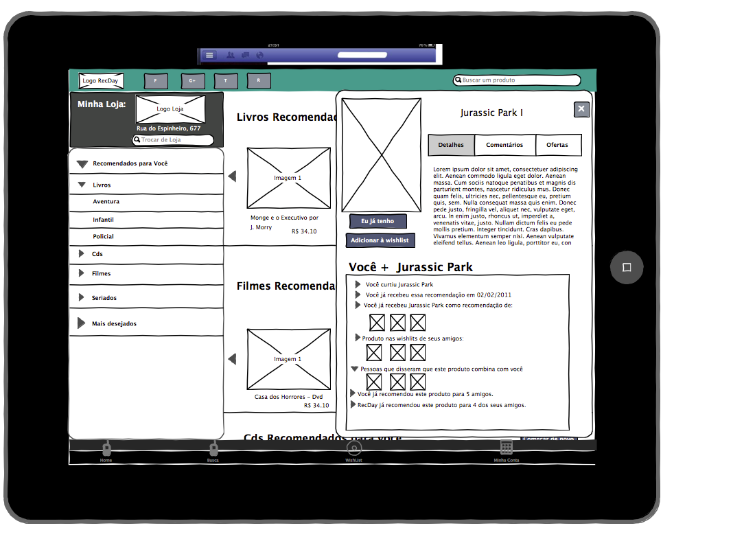
Hybrid Social Context-Aware Recommender RecDay

This hybrid social context-aware recommender (which we call recday) is a engine composed by several modular components, which we employ a broad range of semantic analysis techniques, including information extraction and integration, natural language processing and machine learning. The main task of this recommender is to analyze information about his posts, bios and relationships/lists collected from the social genome and summarize it (all this data would represent the interests of the user) in profiles, which we could call DNA. Those profiles built by the recday would infer the possible interests of the users and would serve as basis for personalized recommendations of products and services from the retail stores/e-commerce applications.

A perfect example for this proccess, which we call the translation, is when you mentioned several times about Apple products (such as macbook, ipod, iphone, etc) at your tweets. Even you never used the word "Apple", we can use the Social Genome to detect the products and infer that you are interested in Apple products. The following figure illustrate certain kinds of entities and relationships collected in the Social Genome:

The relationships extracted from the social web data

The second step of this engine is to build the user profile. Different from another approaches which it only uses the content or the historical data from reviews or ratings from the user, the Recday would go further and would analyze the temporal context included in the interests of the user. Several reports on consumer behavior show that the user desires are influented by external factors and even the humour or feelings of the person at the certain moment. It is required to collect in a stealth way (with the user permission of course) his social data and build his personality defined by several dimensions. Those dimensions represent the current state of the user which may define what kind of suggestions he would like to receive at that particular moment. For example, if you are happy today because you got a new job and posted at your Facebook about that event or even updated your profile about this new position, it would be a valuable information for your DNA profile in order to recommend products and services to celebrate this occasion (You are happy and excited, don't you think ?).

Another important component in this proccess is the product side. We need extract more information from their products portfolio. Items must be juiced in order to get all its meta-data available. Imagine the movie Batman where we have details about the year, genre, cast, production, direction, sinoypsis, etc. All this data can be used to build the DNA Item and be expressed by a collection of dimensions that represent the item profile. With those profiles (DNA User and DNA Item) we compute the similarity between user and items in order to produce a list of top recommendations and related explanations.

The Social Architecure of the Recommender

The final result can be shown in several mediums: mobile apps, widgets, web, API's, pluggins, etc. It is important the usability and how you will present all this information for a particular user. That's why the user interface must be simple and easy to navigate and have mechanisms to collect the user's feedback for the suggestions given by the engine. This proccess is cyclic, so when you give a feedback (a like or dislike or a comment about the suggestion), this piece of information is handled and leveraged to power your DNA profile.

A particular medium of the recommendations: Ipad Demo

In order to build all these interesting technical challenges, we needed to start developing our in-house solution called Crab, which proccesses all this data and employ several analysis and filtering techniques  to deal with the percularities of this heterogeneous sources of data. The first start is the launch of the Deepjewel Labs. Deepjewel is a principle that we can mine the wealth in data, by identifying interesting entities and relationships and converting them into valuable information as input in the recommendation proccess of items and services. 

In summary, all those human and computation techniques can be used to perform a deep semantic analysis of web and social data, where the result for a commerce application or retail store is the ability to offer what the users want before they know that they really want in a personalized way. The RecDay  would be able to daily offer relevant product and services to their customers without they even know it exists. This is a new way to shop in which you don't have to go find products, service and information; the machine will help them find their way to you.

To know more about our Deepjewel labs, visit the website (currently in portuguese):  

http://www.deepjewel.com

I hope you enjoyed,

Marcel Caraciolo

Machine Learning with Python: Meeting TF-IDF for Text Mining

3Hi all,

This month I was studying about information retrieval and text mining, specially how to convert the textual representation of information into a Vector Space Model (VSM).  The VSM is an algebraic model representing the importance of a term (tf-idf) or even the absence or presence (Bag of Words) of it in a document. I'd like to mention the excellent post from the researcher Christian Perone at his blog Pyevolve about Machine learning and Text Mining with TF-IDF, a great post to read.

I decided in this post to be shorter and give some examples using Python . I expect at the end of this post you feel confortamble to use tf-idf at your tasks handling with text mining.

By the way, I extremely recommend you to check the scikit.learn machine learning toolkit. There is a whole package to work with text classification, including TF-IDF with Python!

What is TF-IDF ?

Term Frequency - Inverse Document Frequency is a weighting scheme that is commonly used in information retrieval tasks. The goal is to model each document into a vector space, ignoring the exact ordering of the words in the document while retaining information about the occurrences of each word.

It is composed by two terms: one first computes the normalized Term Frequency, which is the number of times a word appears in a documnet, divided by the total number of words in that document. Then, the second term is the Inverse Document Frequency, which is computed as the logarithm of the number of the documents in the corpus divided by the number of documents where the term ti appears. Or, in symbols:

and 

The TF-IDF gives how important is a word to a document in a collection, since it takes in consideration not only the isolated term but also the term within the document collection. The intuition is that a term that occurs frequently in many documents is not a good discriminator ( why emphasize a term which is almost present in the entire corpus of your documents ?)  So it will scale down the frequent terms while scaling up the rare terms; for instance, a term that occurs 10 times more than another isn't 10 times more important thant it.

For computing the TF-IDF weights for each document in the corpus, it is required in the corpus a series of steps:  1) Tokenize the corpus  2)  Model the Vector  Space  and 3) Compute the TF-IDF weight for each document in the corpus.

Let's going through each step:


Tokenization

First we need to tokenize the text. To do this, we can use the NLTK library which is a collection of natural language processing algorithms written in Python. The process of tokenizing the documents in the corpous is a two steps:  First the text is splint into sentences, and then the sentences are split into the individual words. It is important to notice that there are several words that are not relevant, that is, terms like "the, is, at, on", etc...  aren't going to help us, so in the information extraction, we ignore them. Those words are commonly called stop words and they are present in almost all documents, so it is not relevant for us. In portuguese we also have those stop words such as (a, os , as , os, um , umas, que, etc.)

So considering our example below:

We will tokenize this collection of documents and represent them as vectors (rows) of a matrix with |D| x F shape, where |D|  is the cardinality of the document space, or how many documents we have and the F is the number of features, in our example it is represented by the vocabulary size.

So the matrix representation of our vectors above is:

As you have noticed, these matrices representing the term frequencies (tf) tend to be very sparse (lots of  zero-elements),  so you will usually see the representation of these matrices as sparse matrices. The code shown below will tokenize each document in the corpus and compute the term frequencies.

Model the Vector Space

Now that each of the documents in the corpus has been tokenized, the next step is to compute the document frequency quantity, that is, for each term, how many documents that term appears in. Before going to IDF, it is important to normalize the term-frequencies. Why ?  Imagine that we have a repeated term in document with porpuse of improving its ranking on an Information Retrieval System or even create a bias torwards long documents, making them look more important than they are just because of the high frequency of the term in the document. By normalizing the TF vector we can overcome this problem.
The code.

Compute the TF-IDF

Now that you saw how the vector normalization was applied, we will now have to compute the second term of tf-idf: the inverse document frequency. The code is provided below:

The TF-IDF is the product between the TF and IDF.  So a high weight of the tf-idf  is reached when you have a high term frequency (tf) in the given document and low document frequency of the term in the whole collection. Now let's see the tf-idf computed for each term present in the vector space.

The code.

Putting everything together, the following code will compute the TF-IDF weights for each document. And the result matrix it will be:

A row of this matrix would be:

I ommited the zero-values elements of the row.

If we would decide to check the most relevant words for this place, by using the tf-idf I could see that the place has a nice hot chocolate drink (0.420955 <= chocolate quente ótimo), the soft drink nega maluca is also delicious (0.315716 - nega maluca uma delicia),  its Cheese bun is also quite good (0.252573 - pao de queijo muito bom).

And that is how we comput  our  matrix.  You can take a look at this link and this one to know how to use it with GenSim and Scikit.Learn respectively.

That's all,  I hope that  you enjoyed this article and help more people to know how to implement the tf-idf weight to mine your collection of texts.  Feel free to comment and make suggestions.

The source code of this example is also available.

Regards,

Marcel Caraciolo

Machine Learning with Python - Logistic Regression

 Hi all,

I decided to start a new series of posts now focusing on general machine learning with several snippets for anyone to use with real problems or real datasets.  Since I am studying machine learning again with a great course online offered this semester by Stanford University, one of  the best ways to review the content learned is to write some notes about what I learned. The best part is that it will include examples with Python, Numpy and Scipy. I expect you enjoy all those posts!

The series:

• Linear Regression

In this post I will cover the Logistic Regression and Regularization.

Logistic Regression

Logistic Regression is a type of regression that predicts the probability of ocurrence of an event by fitting data to a logit function (logistic function).  Like many forms of regression analysis, it makes use of several predictor variables that may be either numerical or categorical. For instance, the probability that a person has a heart attack within a specified time period might be predicted from knowledege of the person's age, sex and body mass index. This regression is quite used in several scenarios such as prediction of customer's propensity to purchase a product or cease a subscription in marketing applications and many others. 

Visualizing the Data

Let's explain the logistic regression by example. Consider you are the administrator of a university department and you want to determine each applicant's chance of admission based on their results on two exams. You have the historical data from previous applicants that you can use as a trainning set for logistic regression.  For each training example, you have the applicant's scores on two exams and the admissions decision.   We will use logistic regression to build this model that estimates the probability of admission based the scores from those two exams.

Let's first visualize our data on a 2-dimensional plot as show below. As you can see the axes are the two exam scores, and the positive and negative examples are shown with different markers.

Sample training visualization

The code

Costing Function and Gradient

The logistic regression hypothesis is defined as:

where the function g  is the sigmoid function. It is defined as:

The sigmoid function has special properties that can result values in the range [0,1].  So you have large positive values of X, the sigmoid should be close to 1, while for large negative values,  the sigmoid should be close to 0.

Sigmoid Logistic Function 

The cost function and gradient for logistic regression is given as below:

and the gradient of the cost is a vector theta where the j element is defined as follows:

You may note that the gradient is quite similar to the linear regression gradient, the difference is actually because linear and logistic regression have different definitions of h(x).

Let's see the code:

Now to find the minimum of this cost function, we will use a scipy built-in function called fmin_bfgs.  It will find the best parameters theta for the logistic regression cost function given a fixed dataset (of X and Y values).

The parameters are:

• The initial values of the parameters you are trying to optimize;
• A function that, when given the training set and a particular theta, computes the logistic regression cost and gradient with respect to theta for the dataset (X,y).

The final theta value will then be used to plot the decision boundary on the training data, resulting in a figure similar to the figure below.

Evaluating logistic regression

Now that you learned the parameters of the model, you can use the model to predict whether a particular student will be admited. For a student with an Exam1 score of 45 and an Exam 2 score of 85, you should see an admission probability of 0.776.

But you can go further, and evaluate the quality of the parameters that we have found and see how well the learned model predicts on our training set.  If we consider the threshold of 0.5 using our sigmoid logistic function, we can consider that:

Where 1 represents admited and -1 not admited.

Going to the code and calculate the training accuracy of our classifier we can evaluate the percentage of examples it got correct.  Source code.

89% , not bad hun?! 

Regularized logistic regression

But when your data can not be separated into positive and negative examples by a straight-line trought the plot ?  Since our logistic regression will be only be able to find a linear decision boundary, we will have to fit the data in a better way. Let's go through an example.

Suppose you are the product manager of the factory and you have the test results for some microships  of two different tests. From these two tests you would like to determine whether the microships should be accepted or rejected.  We have a dataset of test results on past microships, from which we can build a logistic regression model.  

Visualizing the data

Let's visualize our data. As you can see in the figure below, the axes are the two test scores, and the positive (y = 1, accepted) and negative (y = 0, rejected) examples are shown with different markers.

Microship training set 

You may see that the model built for this task may predict perfectly all training data and sometimes it migh cause some troubling cases.  Just because ithe model can perfectly reconstruct the training set does not mean that it had everything figured out.  This is known as overfitting.   You can imagine that if you  were relying on this model to make important decisions, it would be desirable to have at least of regularization in there. Regularization is a powerful strategy to combat the overfitting problem. We will see it in action at the next sections.

Feature mapping

One way to fit the data better is to create more features from each data point. We will map the features  into all polynomial terms of x1 tand x2 up to the sixth power.

As a result of this mapping, our vector of two features (the scores on two QA tests) has been transformed into a 28-dimmensional vector. A logistic regression classifier trained on this higher dimension feature vector  will have a more complex decision boundary and will appear nonlinear when drawn in our 2D plot.

Although the feature mapping allows us to buid a more expressive classifier, it also me susceptible to overfitting. That comes the regularized logistic regression to fit the data and avoid the overfitting problem.


Source code.

Cost function and gradient

The regularized cost function in logistic regression is :

Note that you should not regularize the parameter theta, so the final summation is for j = 1 to n, not j= 0 to n.  The gradient of the cost function is a vector where the jn element is defined as follows:

Now let's learn the optimal parameters theta.  Considering now those new functions and our last numpy optimization function we will be able to learn the parameters theta. 

The all code now provided (code)

Plotting the decision boundary

Let's visualize the model learned by the classifier. The plot will display the non-linear decision boundary that separates the positive and negative examples. 

Decision Boundary

As you can see our model succesfully predicted our data with accuracy of 83.05%.

Code

Scikit-learn

Scikit-learn is an amazing tool for machine learning providing several modules for working with classification, regression and clustering problems. It uses python, numpy and scipy and it is open-source!

If you want to use logistic regression and linear regression you should take consider the scikit-learn. It has several examples and several types of regularization strategies to work with.  Take a look at this link and see by yourself!  I recommend!

Conclusions

Logistic regression has several advantages over linear regression, one specially it is more robust and does not assume linear relationship since it may handle nonlinear effects. However it requires much more data to achieve stable, meaningful results.  There are another machine learning techniques to handle with non-linear problems and we will see in the next posts.   I hope you enjoyed this article!

All source from this article here.

Regards,

Marcel Caraciolo