Tools for Machine Learning Performance Evaluation: Confusion Matrix

Hi all, 

I'll start to write some posts starting from now about Supervised and Unsupervised learning, specific related to performance evaluation such as classification accuracy, lift, roc curves, F1-Score and errors.

The Confusion Matrix

Let's start with the one popular tools to evaluate the performance of a model in tasks of classification or prediction:  The confusion matrix (in unsupervised learning it is typically called a matching matrix). Its focus is on the predictive capability of a model  rather than how fast the model takes to perform the classification, scalability, etc.

The confusion matrix is represented by a matrix which each row represents the instances in a predicted class, while each column represents in an actual class. One of the advantages of using this performance evaluation tool is that the data mining analyzer can easily see if the model is confusing two classes (i.e. commonly  mislabeling one as another).

The matrix also shows the accuracy of the classifier as the percentage of correctly classified patterns in a given class divided by the total number of patterns in that class. The overall (average) accuracy of the classifier is also evaluated by using the  confusion matrix.

Let's see a confusion matrix in action by showing an example. Imagine that you have a dataset that consists of 33 patterns that are 'Spam' (S) and 67 patterns that are 'Non-Spam' (NS).  For a classifier trained with this dataset to classify an e-mail as 'Spam' or 'Non-Spam', we can use the confusion matrix to see the classification accuracy based on the training data. In the example confusion matrix below, of the 33 patterns that are 'Spam' (S),  27 were correctly predicted as 'Spams' while 6 were incorrectly predicted as 'Non-Spams' (NB) (achieving an accuracy of 81.8%).  On the other hand, of the 67 patterns that are 'Non-Spams', 57 are correctly predicted as 'Non-Spams' while 10 were incorrectly classified as 'Spams' (an accuracy of 85.1%).  The overall accuracy of the classifier  for predicting both classes given this dataset is evaluated achieving 83%.

Confusion Matrix on spam classification model

However the confusion matrix only tell us how the classifier is behaving for individual classes. When a data set is unbalanced (where the number of samples in one class is significantly more than that in the other class - it happens a lot with Spam/Non-Spam datasets) the accuracy evaluated of a classifier is not representative of the true performance of the classifier. For instance, imagine there are 990 patterns that are 'Non Spam'  and only 10 patterns that are 'Spam' , the classifier can easily be biased towards the class 'Non Spam'.  If the model classifies all the samples as 'Non-Spam', the accuracy will be 99%.  And this is not real indication of the classification's performance. The classifier has a 100% recognition rate for 'Non-Spam'  but a 0% error rate for 'Spam'. Looking at the matrix, the system has trouble in predicting the 'Spam' class, even though the system has to be 99% accurate in its prediction. Given that the prediction of 'Spam' class would be the one of actual interest, only using the confusion matrix to evaluate the model's performance is not enough, but it can give us an insight of how the model is predicting the classes and start to use other metrics that we will explain in the next section.

Confusion Matrix on a unbalanced dataset

The Table of  Confusion

In the Confusion Matrix, for each cell in the matrix we have fields as True Positives, False Positives, False Negatives and True Negatives.  These are defined as:

• False Positive (FP):  Falsely Predicting a label (or saying that Non-Spam is a Spam).
• False Negative (FN):  Missing and incoming label (or saying a Spam is Non-Spam).
• True Positive (TP):  Correctly predicting a label (or saying a Spam is Spam).
• True Negative (TN): Correctly predicting the other label (or saying Non-Spam is Non-Spam).

Looking at the confusion matrix in a general view is as follows:

Confusion Matrix

 
How can we use those metrics ?  For instance, let's consider the previous model now for predicting if a text message have positive or negative opinion associated (common in sentiment analysis task).  We have a data set with 10.000 text messages where the model correctly predicts 9.700 negative messages, and 100 positive messages. The model still incorrectly predicts 150 messages which are positive to be negative, and 50 messages which are negative to be positive.  The resulting Confusion Matrix is shown below.

Confusion Matrix on Sentiment classification task

For the binary classification problems, which was our case situation , we can derive from those metrics two equations called sensitivity and specificity. They are commonly used for the evaluation of any binary classifier. 

The Specificity (TNR) measures the proportion of messages that are negative (TN) of all the messages that are actually negative (TN+FP). It can be looked at as the probability that the message is classified as negative given that the message does not contain negative words. With higher specificity, fewer positive messages are labeled as negative.

On the other hand, Sensitivity (TPR) is the proportion of messages that are positive (TP) of all the messages that are actually positive (TP+FN).  It can be seen as the probability that the message is positive given that the patient contain positive words. With higher sensitivity, fewer actual messages will be classified as negative.  

Sensitivity can be expressed as :

• TP / (TP+FN)

and then Specificity which is:

• TN / (TN+FP)

In general here, Sensitivity means the accuracy on the class Negative, and Specificity means the accuracy on the class Positive. So using these metrics, what is the accuracy on Positive and Negative messages  ?

• Sensitivity = TP / (TP+FN) = 100/(100+50) = 0.4 = 40% 
• Specificity = TN / (TN+FP) = 9700/(9700+150) = 0.98 = 98% 

As you can see, if we have a test for sentiment classification with 40% sensitivity and 98% specificity, and we have to check 1000 messages, and 500 of them are positive and 500 are negative. You are likely to get about 200 messages true positives, 300 messages false negatives,  490 true negatives and 10 false positives. You can conclude that the the negative prediction is more confident, specially based on the high value of specificity and the low level of sensitivity. As you can see it's a important metric for analyzing the performance of your classifier only looking both separated.

The relationship between sensitivity and specificity, as well as the performance of the classifier, can be visualized and studied using the ROC curve, which it will be one of the next posts about this topic.

I've developed some code in Python for evaluating the Confusion Matrix, Specificity and Sensitivity of a classifier here.  Please make the necessary changes for adapting for your classifier. 

That's all,

I expect you have enjoyed!

Cheers,

Marcel Caraciolo

References

Confusion Matrix - Wikipedia
Binary Classification - Wikipedia
Sensitivity and Specificity - Wikipedia 
Confusion Matrix - QSAR World

MapReduce with MongoDB and Python

Hi all,

 In this post, I'll present a demonstration of a map-reduce example with MongoDB and server side JavaScript.  Based on the fact that I've been working  with this technology recently, I thought it would be useful to present here a simple example of  how it works and how to integrate with Python.

But What is MongoDb ?

For you, who doesn't know what is and the basics of how to use MongoDB, it is important to explain a little bit about the No-SQL movement. Currently, there are several databases that break with the requirements present in the traditional relational database systems. I present as follows the main keypoints shown at several No-SQL databases:

• SQL commands are not used as query API (Examples of APIs used include JSON, BSON, etc.)
• Doesn't guarantee atomic operations.
• Distributed and horizontally scalable.
• It doesn't have to predefine schemas. (Non-Schema)
• Non-tabular data storing (eg; key-value, object, graphs, etc).

Although it is not so obvious, No-SQL is an abbreviation  to Not Only SQL. The effort and development of this new approach have been doing a lot of noise since 2009. You can find more information about it here and here.  It is important to notice that the non-relational databases does not represent a complete replacement for relational databases. It is necessary to know the pros and cons of each approach and decide the most appropriate for your needs in the scenario that you're facing.

MongoDB is one of the most popular No-SQL today and what this article will focus on. It is a schemaless, document oriented, high performance, scalable database  that uses the key-values concepts to store documents as JSON structured documents. It also includes some relational database features such as indexing models and dynamic queries. It is used today in production in over than 40 websites, including web services such as SourceForge, GitHub, Eletronic Arts and The New York Times..

One of the best functionalities that I like in MongoDb is the Map-Reduce. In the next section I will explain  how it works illustrated with a simple example using MongoDb and Python.

If you want to install MongoDb or get more information, you can download it here and read a nice tutorial here.

Map- Reduce 

MapReduce is a programming model for processing and generating large data sets. It is a framework introduced by Google for support parallel computations large data sets spread over clusters of computers.  Now MapReduce is considered a popular model in distributed computing, inspired by the functions map and reduce commonly used in functional programming.  It can be considered  'Data-Oriented' which process data in two primary steps: Map and Reduce.  On top of that, the query is now executed on simultaneous data sources. The process of mapping the request of the input reader to the data set is called 'Map', and the process of aggregation of the intermediate results from the mapping function in a consolidated result is called 'Reduce'.  The paper about the MapReduce with more details it can be read here.

Today there are several implementations of MapReduce such as Hadoop, Disco, Skynet, etc. The most famous is Hadoop and is implemented in Java as an open-source project.  In MongoDB there is also a similar implementation in spirit like Hadoop with all input coming from a collection and output going to a collection. For a practical definition, Map-Reduce in MongoDB is useful for batch manipulation of data and aggregation operations.  In real case scenarios, in a situation where  you would have used GROUP BY in SQL,  map/reduce is the equivalent tool in MongoDB.

Now thtat we have introduced Map-Reduce, let's see how access the MongoDB by Python.

PyMongo

PyMongo is a Python distribution containing tools for working with MongoDB, and is the recommended way to work with MongoDB from Python. It's easy to install and to use. See here how to install  and use it.

Map-Reduce in Action

Now let's see Map-Reduce in action. For demonstrate the map-reduce I've decided to used of the classical problems solved using it: Word Frequency count across a series of documents. It's a simple problem and is suited to being solved by a map-reduce query.

I've decided to use two samples for this task. The first one is a list of simple sentences to illustrate how the map reduce works.  The second one is the 2009 Obama's Speech at his election for president. It will be used to show a real example illustrated by the code.

Let's consider the diagram below in order to help demonstrate how the map-reduce could be distributed. It shows four sentences that are split  in words and grouped by the function map and after reduced independently (aggregation)  by the function reduce. This is interesting as it means our query can be distributed into separate nodes (computers), resulting in faster processing in word count frequency runtime. It's also important to notice the example below shows a balanced tree, but it could be unbalanced or even show some redundancy.

Map-Reduce Distribution

Some notes you need to know before developing your map and reduce functions:

•  The MapReduce engine may invoke reduce functions iteratively; thus; these functions must be idempotent. That is, the following must hold for your reduce function:

                 for all k,vals : reduce( k, [reduce(k,vals)] ) == reduce(k,vals)

•  Currently, the return value from a reduce function cannot be an array (it's typically an object or a number)
• If you need to perform an operation only once, use a finalize function.

 Let's go now to the code. For this task, I'll use the Pymongo framework, which has support for Map/Reduce. As I said earlier, the input text will be the Obama's speech, which has by the way many repeated words. Take a look at the tags cloud (cloud of words which each word fontsize is evaluated based on its frequency) of Obama's Speech.

Obama's Speech in 2009

For writing our map and reduce functions, MongoDB allows clients to send JavaScript map and reduce implementations that will get evaluated and run on the server. Here is our map function.

wordMap.js

As you can see the 'this' variable refers to the context from which the function is called. That is, MongoDB will call the map function on each document in the collection we are querying, and it will be pointing to document where it will have the access the key of a document such as 'text', by calling this.text.  The map function doesn't return a list, instead it calls an emit function which it expects to be defined. This parameters of this function (key, value) will be grouped with others  intermediate results from another map evaluations that have the same key (key, [value1, value2]) and passed to the function reduce that we will define now.

wordReduce.js

The reduce function must reduce a list of a chosen type to a single value of that same type; it must be transitive so it doesn't matter how the mapped items are grouped.

Now let's code our word count example using the Pymongo client and passing the map/reduce functions to the server.

mapReduce.py

Let's see the result now:

And it works! :D

With Map-Reduce function the word frequency count is extremely efficient and even performs better in a distributed environment. With this brief experiment we  can see the potential of map-reduce model for distributed computing, specially on large data sets.

All code used in this article can be download here.

My next posts will be about  performance evaluation on machine learning techniques.  Wait for news!

Marcel Caraciolo

References

• http://nosql.mypopescu.com/post/394779847/mongodb-tutorial-mapreduce
• http://fredzvt.wordpress.com/2010/04/24/no-sql-mongodb-from-introduction-to-high-level-usage-in-csharp-with-norm/

CodeCereal : Blog about Logic programming and artificial intelligence!

Hi all,

I'd like to share a great blog that my colleague and friend has started to write about Artificial Intelligence and Reasoning and expert systems: The blog CodeCereal by Daker Fernandes, an undergraduate student from  Informatics Center (CIN) / UFPE .

I've read some posts and it's quite interesting the recently posts about abudctive reasoning, knowledge representation and the building of expert systems using  Prolog.   Anyone interested about this area and logic programming must take a look at this blog!!

Congratulations Daker and keep going with this great work!

Regards,

Marcel

Working on Sentiment Analysis on Twitter with Portuguese Language

Hi all,

In this post I would like to write about my last studies that I was  focusing on. In recent years it is noticeable the increase in amount of information available on the Web. People have started to share in the Web their knowledge and opinions in blogs, social networks and other medium.

On top of that, it have appeared a new research field related to Natural Language Processing, called Opinion Mining also known as Sentiment Analysis. Sentiment Anaylsis aims to identify the sentiment or feeling in the users to something such as a product, company, place, person and others based on the content published in the web. In the view of the requester, it is possible to obtain a full report including a summary about what people are feeling about an item without the need of find and read all opinions and news related to it.

In machine learning area, sentiment analysis is a  text categorization problem which desires to detect favorable and unfavorable opinions related to a specific topic. Its main challenge is to identify how the sentiments are expressed in text and whether they point a positive opinion or a negative one.

There are many applications for the use of Sentiment Analysis, some as follows:

• Sentiment Analysis in Company Stocks :  An important data for investors in order to identify the humor of the market to the companies stocks based on the opinion of analysts, therefore, identifying the trends in their prices.

• Sentiment Analysis in Products: A company might be interested in the opinion of their customers about a certain product. For example,  Google (or another company) can use the sentiment mining to know what the people are speaking about the Android cellphone: Nexus One. This information can be used to improve their products or even identify new marketing strategies.

• Sentiment Analysis on Places:  One person who will travel might want know the best places to visit or the best restaurant to eat. The opinion mining could help those people recommending good places during the planning of their travel.

• Sentiment Analysis on elections: The voters could use the sentiment analysis to identify the  opinion of other voters about a specific candidate.

• Analysis on games and movies:  It is possible to mine the sentiments about games and even movies. We will talk more about this in the future.

Another application for sentiment analysis is on status messages on social networks such as Twitter or Facebook. Twitter has gained a special attention recently where people used it  to express their opinion on certain topic.  Therefore, applying sentiment analysis tools  for Twitter that attempt to classify tweets into either positive, negative or neutral categories  automatically could be quite useful for companies and marketers. It is a widely public data source that couldn't be ignored.

Of course, there are several tools in this area, but more focused on classifying tweets in english language. When using this tools for portuguese comments, many tweets end up in the wrong classification. It happens since those tools are generally trained with algorithms modeled to parse and extract english words. In Brazil, there is a quite interesting web tool called Opsys developed by Thomas Lopes  which is focused on mining opinions from feeds and tweets in the web. Currently, its focus is on brazilian elections 2010 and investments (companies stocks). It works really well with portuguese texts and have a nice web summarization tool for analysis.

But since it is a new area, specially working with portuguese corpora I've decided to develop a simple working sentiment analysis tool for identifying opinions on from Twitter. For this, I apply a common and simple machine learning technique called Naive Bayes to classify the set of tweets related to movie reviews  which I will explain more about it in the next sections.

Ok, But how does the sentiment analysis work ?! What are the required steps ?

1. Data Collection and Pre-processing:  In this step, it is important to search in the web the item of interest, that is, what you want to know the opinion about. It is important also to remove all facts that don't express opinions like news and objective phrases. if your system doesn't identify  subjectivity. The focus is on the user's opinions. The pre-processing is also important in order to remove unnecessary words or irrelevant words to the next step: The classification. 

      2. Classification: The polarity of the content that must be identified. Generally, the polarities used are positive, negative or neutral.

      3.  Presentation of Results: In this step, the classification of several opinions must be summarized in order to be presented to the user. The goal is to facilitate the understanding and give a general comprehension about what people are talking about an item.  This summarization can be expressed in graphics or text. 

Data Collection and Pre-processing

The first step (Data Collection) is related to the information retrieving. It is necessary to extract keywords from the text that may lead to correct classification. Keywords about the original data are usually stored in the form of a feature vector, F = (f1,f2,... fn).  Each coordinate of a feature vector represents one word, also called a feature, of the original text.  The value for each feature may be a binary value, indicating the presence or absence of the feature, an integer which may further express the intensity of the feature in the original text.  It is important to have a good selection of features since it strongly influences the subsequent learning in the machine learning process.  The goal of selecting good features is to capture the desired properties of the original text that are relevant for the sentiment analysis task. Unfortunately, this task for finding best features does not exist. It is required to rely on our intuition, the domain knowledge and a lot of experimentation to choose the best set of features. I strongly recommend the study of the  Natural Language Processing (NLP)  subject, which it may help you to understand this vast research field.

Our approach includes the use of Bag-of-Words. It is a popular model used in Information Retrieving that takes individual words (unigrams) in sentence as features, assuming their conditional independence. So the whole text is represented by a unordered collection of words.  Each feature in the vector represents a existence of one word. The challenge with this approach is the choice of words that are appropriate to become features.

For instance, considering this model, the tweet:  'Assisti hoje o filme Eclipse, ele é lindo !'  may be represented by the following feature vector:

 F = {'Assisti': 1 , 'hoje': 1, 'o': 1, 'filme': 1, 'Eclipse': 1, 'ele': 1, 'é': 1, 'lindo':1}

Here we represent the feature vector as a python dictionary.

Obviously, for any real use, we have to compare this vector to a feature vector that would have much larger number of words. It would be necessary in fact a dictionary of the language, however this model would be inefficient since it would overfit and lead to bad performance when exposed to new examples.

In literature, a common approach is to manually select the most important keywords, for example the word 'lindo' (adjective) is a good indicator of the author's opinion. The most important keywords such as 'excelente',  'horrível', 'fraco'  would be selected as features  since  they express polarity of a sentence). However, Pang et al. show that manual keyword model is outperformed by statistical models, where a good set of words that represent features are selected by their occurrence in the existent training corpus. So, the quality of the selection would depend on the size of the corpus and the similarity of domains of training and test data.  The use of corpus from different domains that don't have the same properties of the domain of the text we want to classify, may lead to inaccurate results. For instance, if the analysis is done on a set of tweets related to a product and is trained with a set based on movies, the most of the sentences would be misclassified.  It is important also to create a dictionary which will capture the most important features for classifying previously unseen sentences.

Additionally, it is possible to remove some of the existing words that bring little useful information like pronouns, articles, prepositions, etc (List of stop words).  Of course, the model presented here is simple, and there are several limitations, which include the inability to capture the polarity relation between words and different meanings of one word.  Another limitations would be suppressed by use of regular expressions for handling the negation and parts of speech for a syntax analysis of the word.

Classification

Classification algorithms are efficient and consolidated techniques for this sentiment classification task, since it predicts the label for a given input. However, depending on which approach used (supervised or unsupervised), it will be required a training set with labeled examples before new tweets be classified. It is important to train the model with the set in a domain related to the data domain that will be used as input. The labels we are interested here are the subjectivity of the sentence and the polarity of the sentence (neutral, positive or negative).  There are several machine learning techniques for this task, but in this article we are using the simplest one but with a great  efficience in classification problems: Naive Bayes technique.

The Naive Bayes model or Naive Bayer classifier is a simple probabilistic classifier based on the Baye's theorem with strong independence assumptions. In simple terms, this probability model assumes that the presence or absence of a particular feature of a class is unrelated to presence or absence of any other feature.  For instance, a car may be considered to be a vehicle if there are  4 tires, engine and at least 2 doors.  Even if these features depend on each other, the naive Bayes classifier considers all these properties to independently contribute to the probability that the car is an vehicle.

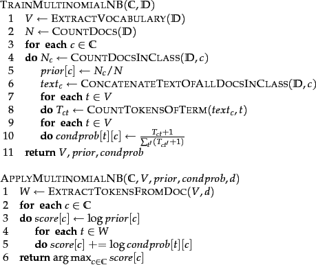
In our case, each stemmed word in a tweet is taken to be a unique variable in the model, and the goal is to find the probability of that word, and consequently the all sentence itself, belonging to a certain class: Positive vs Negative.  In spite of their naive design and simplified assumptions,  naive Bayes classifiers have worked very well in many complex real-word situations. One of the extensive uses is in spam filtering. In fact, one of the most popular packages (SpamAssassin) is a direct implementation of Naive Bayes. It is a an amazingly simple approach and also a powerful classifier.  More information about the algorithm of Naive Bayes it can be found here and here.

In this tutorial I have used the implementation of a simple Naive Bayesian Classifier. There are some variations using Fisher Score discriminant function, which will not be explored in this article now.

In our problem domain, we will use the Naive Bayes classifier to classify the tweets in Positive or Negative.  To apply this task, it is necessary to train the classifier by creating a training set of tweets (or words) already classified (in Positive or  Negative). Trained the model,  Naive Bayes assumes that all features in the feature vector (after the pre-processing step), and applies Bayes' rule on the tweet. Naive Bayes calculates the prior probability frequency for each label in the training set. Each label is given a likelihood estimate from the contributions of all features, and the sentence is assigned the label with highest likelihood estimate, that is, 'Positive' or 'Negative'. 

Summarization

The last step: The presentation of the results. Generally, it can be presented by using text or charts. The summarization in text is not a easy task, and it has a research field only for it. The common presentation is a list of sentences where for each the classification is shown by its side.

Summarization by TwitterSentiment Analyzer  -  http://twittersentiment.appspot.com/

The other common option is to use charts to present the results. It's the simplest way, and there are many flavors for this presentation. And don't forget they are more attractive for the end users and reports.

Summarization by TwitterSentiment Analyzer  -  http://twittersentiment.appspot.com/

Our Study Case:  Movies Reviews on Twitter

For a simple study case and demonstration here, I've created a training set with more about 300 sentences related to movie reviews on Twitter. So sentences such as 'Eu amei o filme Eclipse!' or 'Eclipse poderia ser melhor. #horrível Pior filme da saga.'  are  labeled under positive and negative polarities for creating the training set. It is important to notice that my data corpus are related to portuguese tweets.  So english ones will not work properly.  I've used the Twitter Search API for searching tweets with the keyword 'Eclipse',  the new released  movie in the theaters from the saga  'Twilight' and fetched tweets during three days (July 05th 2010 - July 07th 2010). 

What people are talking about the movie Eclipse on Twitter ??

The task is to analyze the opinions about the movie in Twitter. Using the Naive Bayes Classifier with some adjustments to include the 'Neutral' Classification, we have analyzed 4265 tweets.  I have used some pre-processing techniques explained above. All the code was written in Python. The result you can see in the graph below.

Polarity Chart on tweets about the movie 'Eclipse'

As you may notice, brazilians are really loving the movie Eclipse!! There are also a great amount on neutral tweets, it means that the classifier didn't have the confidence to classify as positive or negative, (I'll explain soon) or tweets that don't express sentiment (opinions).

You can see some of the tweets classified as follows:

Some Tweets classified related to the movie Eclipse

The neutral classification, I've added a simple threshold where after evaluating the probabilities for each polarity (Positive and Negative). The maximum one is compared to a threshold and if its value isn't higher, it is classified as a neutral one. It means that the classifier doesn't have the confidence to classify the tweet as one of the classes trained in the model.

As you can see, the Naive Bayes is a simple machine learning technique quite efficient for automatically extract sentiment from small sentences like Tweets. However, it is important to notice that it still can be improved with new feature extraction approaches or another robust machine learning techniques.

Demo

Soon I will provide all the source code for this project, but if you want to play around with the classifier, I've developed a simple REST API for using the classifier for simple tests. This version is still not official and it only works with movie reviews domain (in portuguese of course).

Docummentation 

The output result is in JSON. PLEASE THIS API is still in development. So if you plan on integrating this API into a product, please let me know , so that I can contact you in order to help you to create your own.

The classifier is only working with a single arbitrary text (in portuguese language)  and as result give you its polarity. Example:

Query:

http://mobnip.appspot.com/api/sentiment/classify?text=Encontro+Explosivo+filme+ruim+Danado&query=encontro+explosivo

Response:

{"results": {"polarity": "negativo", "text": "Encontro Explosivo filme ruim Danado", "query": "encontro explosivo"}}

Parameters:
- text: The text you want to classify. This should be URL encoded. 

- query: The subject. This should be URL encoded. (optional)

Response:
- text: original text submitted
- query: original query submitted
- polarity. The polarity values are:
       -  'negativo': corresponds to negative
       -  'neutro': corresponds to neutral
       - 'positivo': corresponds to positive

Conclusions

As we can notice that sentiment analysis is a trend in the Web, with several interesting application with a lot of data sources provided by users.  Microblogs and Social Networks such as Twitter, Facebook and Orkut and another web services are powerful crowding sources for obtain opinions from the users in the Web about any subject and specially to help to answer the question about what people are interested on. Despite the challenge, more companies and researchers are working in this area until one day it would be easy for users and companies to simply obtain complete and rich summarized reports about the opinions from the Web in order to support them in the decision making process in their daily life.

 In machine learning topics, there are also a lot of improvements that would be made for this task and several challenges for researchers to extend it. I would say the most important ones are related to the natural language processing, which is directly associated to sentiment analysis. I would cite the subjectivity identification (distinguish if a text is really a opinion or a fact), identification  of sarcasms, which are not easy to extract,  the multiple reference of items in a same sentence (a tweet referencing Iphone and Ipod) and with different opinions, which it may confuse the classification. Misspelling words and abbreviated words (common in blogs and social networks) are also difficulties for search and classification. Many others could be cited here but it may be found if you search on Google about sentiment analysis.

In the end, I would tell that applying sentiment analysis in portuguese language is still a new area with great challenges to deal with text mining since the language is different from the current ones applied on english in the literature. My work is  a initial discussion about how we can learn more about sentiment analysis and how portuguese could be inserted in this context.  More analysis and a better evaluation should be applied to compare another popular machine learning techniques with Naive Bayes classifier.

I expect   you have enjoyed this tutorial, it's quite long but I believe it could be a useful start for the beginners in machine learning.

Thanks,

See you next time!

Marcel Caraciolo

WordTree: Visualization Tool for Twitter

Hi all,

It has been a while since my last post. But, I am still alive!! In this post I'll be talking about one of my last projects based on natural language processing (NLP) that I've developed: A Visual Word Tree.

But what is a Word Tree ?

A word tree is a visual analyzer tool for unstructured text, such as a article, speech or a book. It is also a new visualization technique that makes easy the exploration of repetitive context. The main idea behind it includes the concordance principle.

Concordances have been used for centuries at biblical scholars to see how different words occur in religious texts. It is a special type of indexation technique, which shows near to each word some words that appears before or after that one. For instance, consider the phrase "if love" in Romeo and Juliet which occurs three times:

As the figure shown above, you will notice that in the words following 'if love' there are many repeated phrases. For example, "be" follows "if love" in all three cases. And "be blind" follows in two cases. To create a word tree, the computer merges all the matching phrases, as in this diagram:

As you can notice, this diagram has a shape of a tree of each node represented by a word, which can be easily interpreted and visualized. It emphasizes in the interactive exploration of short texts (like the short texts of the Bible). This visualization is called WordTree and is based on a well-known data structure in computer science: suffix tree (introduced in the 70's).

IBM scientists have developed a interactive graphical tool, which recently at TEDx São Paulo, Fernanda Viegas from IBM have lectured a great keynote about data visualization techniques, presenting the application of the wordTree technique. The tool is also available for public and for free use at the website ManyEyes.

But why did i developed one ?

One of the problems of ManyEyes is its forbidden use for commercial applications and based on what I've researched there is also a maximum limit of words supported by the tool. I've found other ones like the ManyEyes, but unfortunatelly was not open-source or not available for public.

Therefore, I decided to build my own implementation of concordance based on the suffix tree. Different from the ManyEyes tool, my goal is to create automatically word trees from statuses from the web microblog Twitter. I was inspired by the work done by the Vettalabs who have developed a wordTree for Twitter in Java.

Twitter has a powerful mechanism called Re-Tweet (RT) which can be used by users to repeat any tweet that was already posted by someone, in order to reinforce or support that tweet and spread to all your followers (Making a RT of a tweet you're announcing that tweet for more people in order to see it). The more the number of RT's , the more divulged that tweet had.

Thus, I've developed a simple system that monitors the Twitter in real-time, seeking for tweets that has keywords specified by the users. Furthermore, for each n tweets found, one new tree is created, which shows in a easy way what it has been discussed about that topic, i.e., related to that keyword.

Let's see an example: I've collected some tweets about the recently launched movie in the brazilian theaters: Robin Hood. The figure below illustrates the new word tree created:

WordTree related to the movie Robin Hood

As you can notice, the quantity of tweets processed can be huge - thousand of items in one day. So I decided to prune the tree in order to present only relevant information. For that, we can use some natural language processing techniques such as to choose only nodes that have verbs in the second node and a subject in the first node of the tree. This could simplify the tree and focusing on the texts that have a subject + verb in the beginning (action of the keyword), etc.

The tree presented above is a reverse tree, which shows the words that precede a keyword.(trees with higher depth). The other one is the basic tree where the keyword is the subject:

WordTree related to Brazil ( a mention to the Soccer World Cup)!

Both the suffix tree and the graph was developed using Python programming language. The most interesting part is that you can easily visualize/extract information in real-time on Twitter with this visualization tool. It also summarizes repeated words by increasing its font/letter size so the user can directly understand in a intuitive way, specially in a environment with lots of text and information.

I'd like to mention Murilo Queiroga who has given me some tips to this work. Thanks Murilo!

See you next time,

Marcel Caraciolo